Motif Kernel / SVM Tutorial

This Tutorial shows how you can combine the motif kernel of the strkernel package with a Support Vector Machine (SVM) to predict the cell population based on the motif content of a read sequence.

There are two FASTA files from two different cell populations filled with sequences. If you are not familar with the FASTA format, here is a short explantion. fibroblast.fa are sequences obtained from fibroblast while stemcells.fa contains sequences from stemcells. The goal of this tutorial is to show that we can use prior knowledge to construct motifs and use those motifs to classify new sequences into the two cell populations. The accuracy of the prediction is in this case secondary as long as we get a result that shows that we can use the motif content of sequences to compare their similarity and therefore classify them.

First, you will need some packages for preprocessing, classification and to plot the results.

# preprocessing
import numpy as np
from Bio.Seq import Seq
import Bio.SeqIO as sio

# SVM
from sklearn.svm import SVC
from sklearn.model_selection import train_test_split
from sklearn.metrics import classification_report

# ROC and precision-recall curve
from sklearn.metrics import roc_curve, auc, precision_recall_curve, average_precision_score

# plotting
import matplotlib.pyplot as plt  # plotting

# motif kernel
from strkernel.motifkernel import motifKernel

Preprocessing

In order to use the data with the SVM provided by sklearn we need to read in the FASTA files with Biopython and add some labels. In this case we will label the stemcells as positive (1) and the fibroblast as negative (0).

# load the data
# stemcells
pos_data = [seq.seq for seq in sio.parse('notebook_data/stemcells.fa', 'fasta')]
# fibroblasts
neg_data = [seq.seq for seq in sio.parse('notebook_data/fibroblast.fa', 'fasta')]

pos_labels = np.ones(len(pos_data), dtype=int)
neg_labels = np.zeros(len(neg_data), dtype=int)

y = np.concatenate((pos_labels, neg_labels), axis=0)

Motifs

Now we have to decide which collection of motifs we will be using to construct the motif kernel. There are specific transcription factors binding sites which tend to be enriched in one of the groups. Naturally not every sequence contains the binding site for these transcription factors but we should be able to correctly classify those that do. In stemcells, we expect the oct4 binding site to be enriched because this protein has been shown to be heavily involved in the pluripotency of cells. In fibroblast lung tissue on the other hand, we expect the mafk binding site to be enriched.

The jasper database allows to check for the binding motifs of the transcription factors. If we search for oct4 and mafk we get the following binding sites:

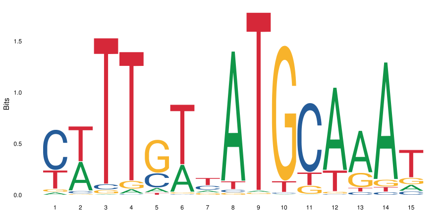
oct4

mafk

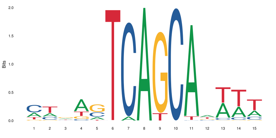
We can now add the most prominent motifs of these bindings sites to our motif collection. For this tutorial we chose the motif TCAGCA of the mafk binding site and the motifs ATGCAA and TTGT of the oct4 binding site. Since the reads originate from both strands we also have to include the reverse complement of the motifs.

In normal use cases the number of motifs is usally a lot higher but for this tutorial the six motifs will be enough.

motif_collection = ["TCAGCA","TGCTGA","ATGCAA","TTGCAT","TTGT","ACAA"]

#create the motif kernel
motif_kernel = motifKernel(motif_collection)

#use the motif kernel to compute the motif content matrix for all sequences
motif_matrix = motif_kernel.compute_matrix(pos_data + neg_data)

Classification

We can now split the matrix into test and training data. The training data can then be used to train the SVM. We will keep 30% of the data as test data to evaluate the model.

#split the data into test and training set
X_train, X_test, y_train, y_test = train_test_split(motif_matrix, y, test_size=0.3, random_state=42, stratify=y)
#train the classifier
clf = SVC()
clf.fit(X_train, y_train)

SVC(C=1.0, cache_size=200, class_weight=None, coef0=0.0,
  decision_function_shape='ovr', degree=3, gamma='auto', kernel='rbf',
  max_iter=-1, probability=False, random_state=None, shrinking=True,
  tol=0.001, verbose=False)

Results

The only thing left to do is to analyze the trained model. sklearn provides a function which can be used to produce a classifcation report. This report shows us the precision, recall and f1-score when we apply the model to our test data. We will also plot the ROC and PRC but first we will have to define a couple of wrapper functions.

def plot_roc_curve(y_test, y_score):
    '''Plots a roc curve including a baseline'''
    fpr, tpr, thresholds = roc_curve(y_test, y_score)
    roc_auc = auc(fpr, tpr)

    plt.figure()
    lw = 2
    plt.plot(fpr, tpr, color='darkorange',
             lw=lw, label='ROC curve (area = %0.2f)' % roc_auc)
    plt.plot([0, 1], [0, 1], color='navy', lw=lw, linestyle='--')
    plt.xlim([0.0, 1.0])
    plt.ylim([0.0, 1.05])
    plt.xlabel('False Positive Rate')
    plt.ylabel('True Positive Rate')
    plt.title('Receiver operating curve')
    plt.legend(loc="lower right")
    plt.show()


def plot_prec_recall_curve(y_test, y_scores):
    '''Plots a precision-recall curve including a baseline'''
    precision, recall, thresholds = precision_recall_curve(y_test, y_scores)
    average_precision = average_precision_score(y_test, y_scores)
    baseline = np.bincount(y_test)[1] / sum(np.bincount(y_test))
    plt.figure()
    plt.step(recall, precision, color='b', alpha=0.2,
             where='post')
    plt.fill_between(recall, precision, step='post', alpha=0.2,
                     color='b')
    plt.axhline(y=baseline, linewidth=2, color='navy', linestyle='--')
    plt.xlabel('Recall')
    plt.ylabel('Precision')
    plt.ylim([0.0, 1.05])
    plt.xlim([0.0, 1.0])
    plt.title('2-class Precision-Recall curve: AP={0:0.2f}'.format(
              average_precision))
    plt.show()


def reportclassfication(clf, X_test, y_test):
    '''Reports classification results with the given model and testdata'''

    print("Detailed classification report:")
    print()
    y_true, y_pred = y_test, clf.predict(X_test)
    print(classification_report(y_true, y_pred))
    print()


# get classfication results with the tuned parameters
reportclassfication(clf, X_test, y_test)

y_scores = clf.decision_function(X_test)
# plot ROC
plot_roc_curve(y_test, y_scores)

# plot PRC
plot_prec_recall_curve(y_test, y_scores)

Detailed classification report:

             precision    recall  f1-score   support

          0       0.77      0.65      0.70      1200
          1       0.70      0.80      0.75      1199

avg / total       0.73      0.73      0.72      2399

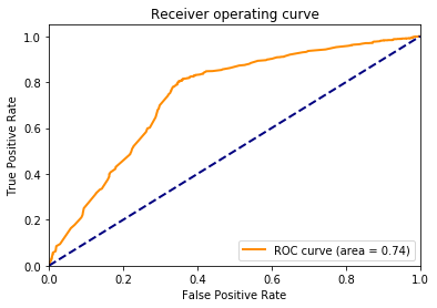
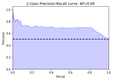
We are able to correctly classify around 80% of the stemcell sequences and 70% of the fibroblast sequences. Obviously this is not the best classification results one could have but we can see that the motifs we derived from the bindings sites of transciption factors can be used to classify sequences into cell populations.

In this example we only used the binding sites of two transcription factors to create a motif collection. For better classifcation results you could include more prior information about the cell populations to extend the motif collection.